
Before You Start
To get the most out of this tutorial, you need a Windows 11 PC to use the Xentara Workbench and a Linux-based computer (a Raspberry Pi or similar hobbyist small computer will work) to install Xentara on. You can also install on a remote or headless system by SSH tunnelling into the target system and following the instructions on the command line of the remote system, however, this walkthrough does not explain using SSH.
If you do not have a Linux computer available, you can use the Windows Subsystem for Linux (WSL). Information on how to install and use WSL can be found online. Please note that to run Xentara in WSL, we recommend installing a Debian distribution.
This document assumes that the user is familiar with the basics of Linux and knows how to operate a command line interface (CLI).
Procedure
The following steps guide you through the entire process:
- Download and install Xentara
- Activate a free trial license
- Get the sample model file and run it in Xentara
- Use the Xentara Workbench to inspect and understand the model
- Optional: Make changes to the model using the Workbench and observe the effects
Installation and Activation
To receive your free version of Xentara, first go to the trial license page:
👉 Click here for your free Xentara trial license
Simply follow the instructions on the page to register for an account, install Xentara for Linux and activate your free trial license.
The Xentara Model File
At the heart of every Xentara-powered application is the so-called model file. This file is created in the well-known JSON markup format (you can learn more about JSON on the internet) and defines:
- the components Xentara should interact with
- the tasks and operations required in the application
- their data relationships with each other
- and the timing behavior via the timing model
But you’ll never need to edit the JSON code directly. All functions of the model are editable in the Xentara Workbench.
Acquiring and Loading the Sample Model File
An example model file with a simple signal generator application can be found at this link:
👉 Click here for the sample Xentara model file
You can right click this link in your web browser and select “Save As” to download the model to your computer. Now you have to make sure it is stored in the right place for Xentara to find. On startup, Xentara automatically searches for the model file in predefined directories. Under Linux, the following paths are checked one after the other until a file named model.json is found:
- ${HOME}/.config/xentara/model.json
- /etc/xdg/xentara/model.json
So make sure to save the sample model in the {HOME}/.config/xentara/ folder with the name “model.json”. Now, you can start Xentara from the command line with the simple command “Xentara”.
When Xentara is started, various startup information is displayed in the console:
- License information: first, details about the license that has just been created and activated are displayed.
- Installed Skills: Xentara then lists all installed skills. This also includes skills that are available but not configured in the current application.
- Information on security, authentication and user configuration
- The path and name of the loaded model file
Since the provided sample model is set to output new data twice a second, you will probably not have time to read these before they scroll off screen, but believe us, they are there.
Below this, you will start to see a lot of data. These are all values from the various function generators. Note that the data does not only contain the current value of each signal, but also attributes like signal quality and the time the signal was last updated. Every data entry you see also has a precise timestamp.

The Xentara Workbench
The Xentara Workbench is available in the download area of the Xentara website and can be installed under Windows:
👉 Click here to download the Xentara Workbench
Download and install the Workbench, then use it to open the model file you downloaded earlier. We’re going to analyze the model, look at its different components and examine how they work.
💡 Good to know: Every element in the Workbench’s configuration area has a small question mark besides its name. A short explanation of the individual parameters can be accessed by clicking the question mark button on the respective object. The top right corner of the tooltip that opens also contains a link to that specific element’s description in the Xentara developer documentation.
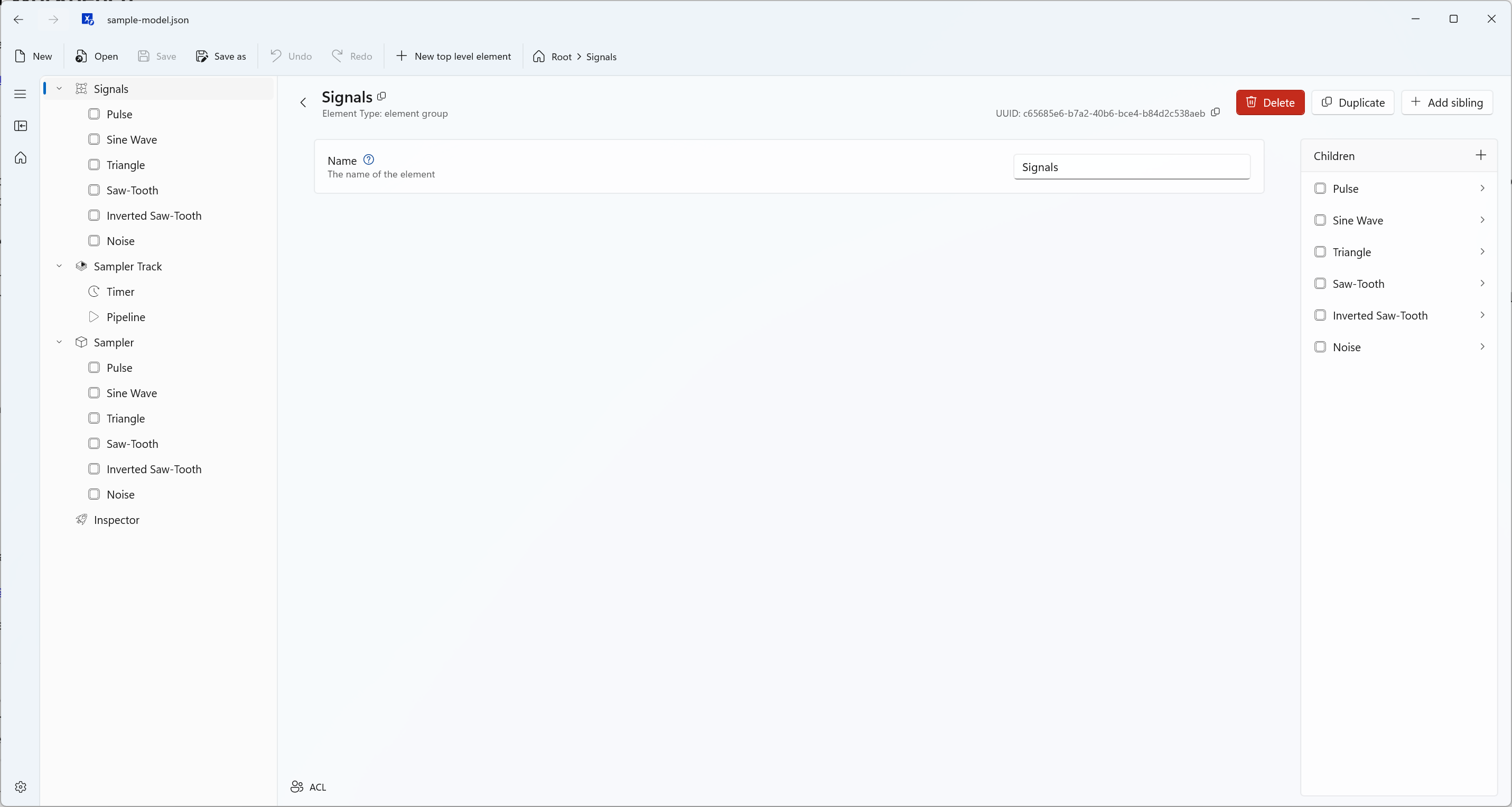
Elements of the Model File
As you can see, the model has four main elements, three of which also have child elements (you may have to click on the little arrows left of the main elements in the tree view to expand their children). “Signals” is a group of data points, “Sampler Track” is our timing model based scheduler, “Sampler” is the signal generator with a list of signals underneath it, and finally the element called “Inspector” is a built in Xentara service that allows you to output values directly to the CLI. (not to be confused with the upcoming graphical Xentara Inspector tool). We are going to look at each element in detail.
We will not be going top to bottom because it is important to understand the Signal Generator first before looking at the Data Points.
Signal Generator
A signal generator labelled “Sampler” is configured in the lower section of the object tree. The signal generator is an integrated function of Xentara for generating cyclic signal curves. Supported signal types include:
- Sine
- Pulse
- White noise
- Triangle
- Sawtooth
Further information about the signal generator is available in the Xentara documentation:
👉 Detailed documentation for the Xentara signal generator
When a Signal is selected in the Workbench, a specific configuration page opens with the associated parameters:
- Waveform – Selection of the signal type (e.g., sine, pulse, triangle...)
- Period duration – Time period of the signal
- Phase offset – Shift of the signal along the time axis
- Pulse width – Proportion of the high phase (only for pulse-like signals)
- Data type – The mathematical type of the generated values (e.g., integer, float...)
- Limit values – Definition of upper and lower limits for the amplitude
By varying these parameters, signal shapes can be specifically adjusted or new variants derived.
💡 Note: The accuracy of the signal generator is determined by the configuration of the associated timing model. For example, if a period duration of 5 seconds is configured, the resulting precision depends on the clock rate at which the timing model executes the signal generator. Since the clock rate in this example is set to 500 ms, a period duration could last up to 5.5 seconds.
Data Points
The elements displayed in the upper area of the object tree in the Workbench are called data points. At first glance, they resemble the variables of the signal generator. In fact, the values of the signal generator variables are reflected in these data points without any time loss. However, the variables within the signal generator are permanently linked to it, while data points represent the I/O points of the technical level but can be freely placed within the hierarchical data model.
As complexity increases, there is a need for a semantic level that allows a more abstract view of the data. This level serves to map data structures in such a way that the underlying technical architecture can be represented in a significantly simplified form. The result is a semantic model that abstracts and thus simplifies the underlying technical architecture.
This hierarchical structuring is built using element groups – in the application example there is a group called “Signals”. These enable data points and tasks to be structured according to the developer’s and user’s needs.
Further information on data points and element groups is available in the Xentara documentation:
👉 Detailed documentation for Xentara data points
👉 Detailed documentation for Xentara element groups
Debugging Inspector
The easiest way to make the generated variables visible in the application example is to use another built-in Xentara function – the internal "Debugging Inspector". This service can read data directly from the signal generator or the associated data points and display it on the command line interface (or your system’s StdOut if configured differently).
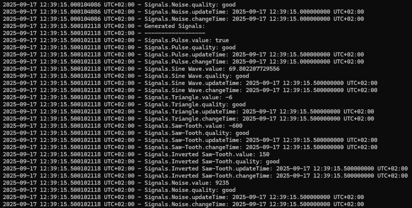
As shown in the example, a data point from the Element Group “Signals” is linked here. Not only can the current attribute Pulse.Value be selected, but also all other available attributes of the data point, such as the time of the last update (Update.Time).
At runtime, Xentara generates the following output based on the configuration shown:
Scheduling
As already mentioned, the signal generator is executed via the timing model. A more in-depth understanding of this can be found in the chapter Scheduling Tasks in the Xentara documentation.
A timing model usually consists of three elements, as shown in the Workbench:
- Track – top instance of an independent timing object
- Pipeline – groups the individual tasks
- Timer – necessary if cyclic activation is to take place
In the sample model shown, a timer is used that is executed periodically every 500 ms. Task activation is already set to Precise in the parent track (Sampler Track) (see Timing Precision (Linux only)). Further measures, such as explicit core allocation, have been omitted in this example.
To activate tasks such as the signal generator and the inspector in the correct sequence, an execution pipeline is required. It determines the order (parallel or sequential) in which the corresponding tasks are executed and the sources through which activation is to take place. In this case, there is a pipeline containing two tasks: "Sampler.generate" and "Inspector.dump". After activation by the timer, the signal generator first generates the data. This data is then read and output by the Debugger Inspector via the linked data points.
💡 Note: As a real-time technology, Xentara is designed to execute processes with minimal latency. Therefore, a single thread handles both the execution of the signal generator and the inspector without a context switch. This avoids the usual time gaps of at least 3–10 µs.
Optional: Making Changes to the Model
Now that you know how to use the Xentara Workbench and have an understanding of some of the elements of the data model, let’s have some fun.
- Change the value ranges (Top and Bottom) of some of the Signals and see how the outputs change.
- Remove or add more signals to your signal generator. Try removing the Noise signal and replacing it with another Sine Wave, for example.
- Change the output by removing the “quality” attributes from the Inspector. This way, you will only see the values that actually change, since signal quality will always be “good”.
- You can change the speed of the output by adjusting your timer. Set it to a longer cycle (e.g. 5 seconds) to make the output slow down, or a shorter cycle to make it go faster.
Keep in mind that for any change to take hold, you have to stop Xentara (this can be done with the key combination “CTRL-C”) and restart it (type in “Xentara”) after saving the changed model file in the default path.
Next Steps
Check out this follow-up guide that shows you how to write your first own Xentara application: