
Before You Begin
To get the most out of this tutorial, you need a Windows 11 PC to use the Xentara Workbench and a running Xentara installation (this can be on a dedicated Linux machine, in WSL, or Xentara installed on Windows). This guide assumes that the user knows how to operate a command line interface (CLI) on Linux or the Windows Powershell.
If you have never installed or run Xentara before, please consult our guide “Installing and Running Xentara for the First Time” first.
👉 Xentara Knowledge Base: Installing and Running Xentara for the First Time
Procedure
The following steps guide you through the entire process:
- Create a simple model file from scratch that contains all necessary information for the application
- Run Xentara to test the created model
The Xentara Model File – A Short Reminder
At the heart of every Xentara-powered application is the so-called model file. This file is created in the well-known JSON markup format (you can learn more about JSON on the internet) and defines:
- the components Xentara should interact with
- the tasks and operations required in the application
- their data relationships with each other
- and the timing behavior via the timing model
But you don’t need to edit the JSON code directly. All functions of the model are editable in the Xentara Workbench.
For those who want to know more, all relevant information on the topic of model files can be found in the official developer documentation:
👉 Detailed documentation on the Xentara model file
The Xentara Workbench
The Xentara Workbench is available in the download area of the Xentara website and can be installed under Windows:
👉 Click here to download the Xentara Workbench
After launching the Workbench, you will be greeted by an empty model and a choice of available objects:
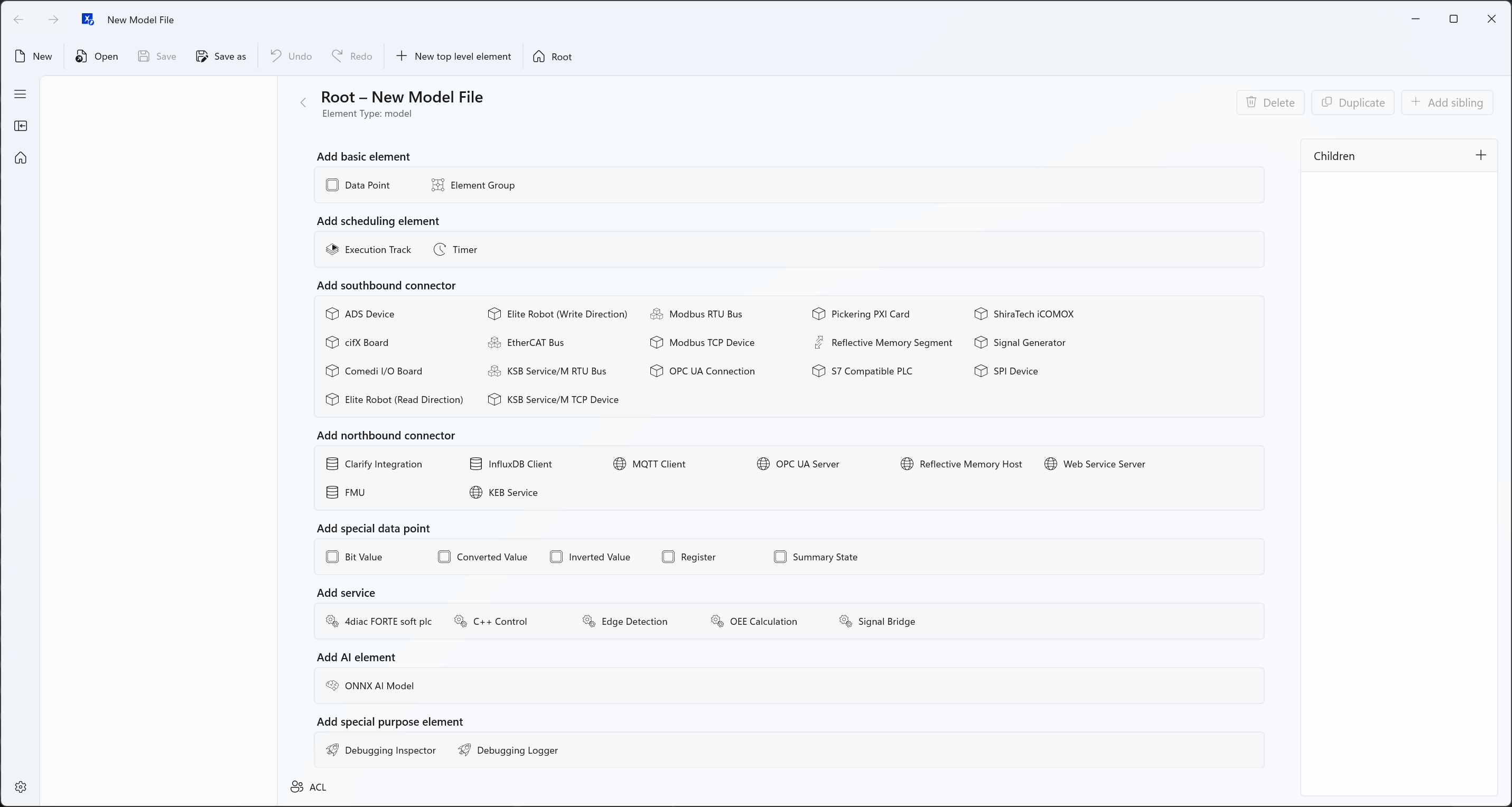
Now, let’s start to build our application.
Creating the Model
Signal Generator
First, we will add our signal generator. Click on the “Signal Generator” object on the screen. The Workbench will then allow you to change the name of the object. For now, let’s stick with the default name of “Generated Signals”.
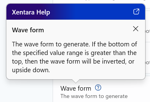
💡 Every element in the Workbench’s configuration area has a small question mark besides its name. A short explanation of the individual parameters can be accessed by clicking the question mark button on the respective object. The top right corner of the tooltip that opens also contains a link to that specific element’s description in the Xentara developer documentation.
Now that the generator is in place, we can add the signals it will put out. Click on the “+” sign besides “Children”. This button allows you to add child elements to any element in the model that supports children. The only object type allowed as a child of the signal generator is called “Signal”. Click on that to add our first signal. You will see a screen where you can define the signal’s parameters.
Our first signal should be a square pulse. Enter the following parameters:
- Name: Pulse
- Data type: Boolean (that means the value can only be 1 or 0, nothing in between)
- Top: 1
- Bottom: 0
- Wave form: Pulse
- Period: 5 s
- Phase offset: 0
- Pulse width: 2,5 s
This will create a square pulse wave signal that switches between 1 and 0 every 2,5 seconds.
To add a second signal, click on “Add sibling” to create another child object of the same parent (in this case, the signal generator). Again, you can only select the type “Signal”. For our second signal, use the following values:
- Name: Wave
- Data type: 64 bit floating point number
- Top: 100
- Bottom: -100
- Wave form: Sine wave
- Period: 15 s
- Phase offset: 5 s
💡 Note that unlike the pulse signal, the “Pulse width” parameter is not available because a sine wave does not have variable pulse width. The Workbench will always offer only those parameters that fit the object type.
If you like, you can add more signals in the way described above.
Creating and Connecting Data Points
While our signal generator only creates a few signals, data models can get very large very quickly. Therefore it is best to organize all variables in our semantic model. For this purpose, we use Data Points. We are going to create DPs for our signals and group them together for easier reference.
First, go back to the top of the data model by clicking on “Root” in the breadcrumbs above the details pane or the house icon in the left toolbar. You are now back at the “root” of the model, from where all other elements grow. Click on “Element Group”. Again, this object offers very little customization; only the name can be changed. Call it “My Signals”.
Now, as we did when adding Signals to the Signal Generator, click on the “+” button to add a child element, then select “Data point”. Use the following parameters for the first one:
- Name: Pulse
- Display name: Current value of the pulse wave
The Display name is a way to give a data point a user facing descriptive name. This allows you to help the user understand the data. - Units: no units
You can use this to add a unit to a value to make it more human readable, like Ampere for electrical currents or psi for pressure value. Since our signals are just numbers, we don’t need a unit designation.
Now it gets interesting, and you will see how the Workbench helps you bring the different parts of your application together. Click in the entry field called “Input/Output”. The Workbench will automatically offer a list of all appropriate elements in the current model that can provide I/Os for our data point. In this case, since the model only contains the signal generator, its name “Generated Signals” will be the only one you can select. After you do that, you will be presented with a choice between all the signals you have created for the generator. In this case, the choice only goes two levels deep (Signal generator and individual signals), but the Workbench can display very complex constructs. Click on “Generated Signals.Pulse” to select the correct signal for input.
💡 Note that the period character (“.”) is used as the delineator between the levels of the data model. So “Generated Signals.Pulse” means that “Pulse” is a child object of “Generated Signals”.
Again, click on “Add sibling” and follow the same instructions to add a data point for the since wave (and any other signals you may have created).
Creating the Output
Of course, we want to see the output of our signal generator to verify that the application is working. To do this, we add a simple output to the command line using the "Debugging.Inspector" element (not to be confused with the upcoming graphical Xentara Inspector tool). This is a built in Xentara service that allows you to output values directly to the CLI.
💡 Note: Using this internal service to dump values directly to the command line is not recommended in actual projects, but for the purposes of this guide, it is a quick and easy solution.
Instead of navigating back to the root of the model, just click on “+ New top level element”. This allows you to add elements directly beneath the root of the model no matter where you currently are. Select the element type “Special > Debugging Inspector”. You can leave the name as it is. For the title, choose something descriptive like “Values of the generated signals:”.
Now we get to add attributes. For this, you can click on the “Add attribute” button or the “+” sign in the attribute list (which is currently empty). As soon as you add an attribute, a screen with its parameters appears. Note that the attribute is not given a name; it is simply a pointer for the debugger telling it what values to display. Click in the Attribute field and you will be presented with a multi-level choice like when choosing the I/O for a data point. Since out data point group is called “My Signals”, select that. You will now see a longer list of choices than before. That’s because the “My Signals” group element has several attributes of its own. At the end of the list will be the group’s children. Select “My Signals.Pulse” and you will see a list of all attributes of the data point we named “Pulse” in the “My Signals” group. Select “My Signals.Pulse.value” (you may have to use the mouse wheel to scroll down the list of attributes) since we want the output to show the current value of the signal.
Now add entries for all other data points you have created. Note that since an attribute is not a model element, you can not use the “Create sibling” function to add more attributes. Instead, navigate back to the Inspector either by clicking it in the tree view on the left of the window or the back button to the left of the attribute’s name, then click on the “Add attribute” button or the “+” sign in the attribute list to add another attribute.
💡 Note: You could also directly use the Signals as attributes (e.g. "Sampler.Sine Wave.value"). However, for this example, we are using the Data Points as this is a more elegant and future-proof solution.
The Timing Model
We now have a signal generator, data points to receive the signals, and a function to display the values. But they aren’t doing anything. That is because tasks in a Xentara application don’t just launch themselves; they need to be triggered by the timing model. For this introduction, we will build a very basic timing model that only triggers our tasks cyclically.
Start by navigating to the root of the model and adding an element with the type “Execution track”. Give it the name “Simple Cycle” and ignore all other parameters – these are for building advanced real-time applications.
Now add a child of the type “Timer” to your track. Set its Period to 500 ms and leave the other parameters as they are. This will ensure that once we start our application, the timer will trigger the tasks associated with it every 500 milliseconds, or twice per second.
Go back to the track and add a “Pipeline” underneath it. The pipeline is the element that actually defines what tasks are launched by each trigger. First, click on “Add trigger”. Choose the Trigger event from the dropdown menu. There are some elements in here that you may not associate with timing. These are used for event-based triggers, which goes beyond the scope of this simple guide. In our case, select “Simple Cycle.Timer.expired”. This ensures the tasks in the pipeline are activated every time the timer expires, i.e. after every cycle.
Now, navigate back to the pipeline again and click on “Add segment”. The segment contains the actual instructions that are performed when the trigger activates. Ignore the checkpoints and click on “Add task”. Again, the Task can be selected from the data model through a dropdown menu. Notice that this dropdown offers only two choices; that is because there are only two elements in our model that can activate tasks. First, select “Generated Signals generate”. This command will tell the signal generator to create current values for all signals that are then automatically linked to their respective data points. Click on the “+” sign to add another task and select “Inspector.dump”. This is the command that tells our debugger to dump the values it currently sees in the system to its output, i.e. the command line.
Starting Xentara
On startup, Xentara automatically searches for the model file in predefined directories. Under Linux, the following paths are checked one after the other until a file named model.json is found:
- ${HOME}/.config/xentara/model.json
- /etc/xdg/xentara/model.json
So make sure to save your newly created model in the {HOME}/.config/xentara/ folder with the name “model.json”. Now, you can start Xentara from the command line with the simple command “Xentara” and you should see the output of our signal generator.
Congratulations, you have just built your first Xentara application!
Optional: Making Changes to the Model and Expanding the Application
Now that you know how to use the Xentara Workbench and have an understanding of some of the elements of the data model, let’s have some fun.
- You can add more signals to your signal generator. The Noise signal e.g. is a purely random signal. Remember to add a data point for every signal you add and then add that data point to the Inspector element.
- You can change the speed of the output by adjusting your timer. Set it to a longer cycle (e.g. 2 seconds) to make the output slow down, or a shorter cycle to make it go faster.
- You can display more information about your signals. For this, go to the Debugger.Inspector element and simply add more attributes. For example, “Generated Signals.Pulse.changeTime” will display the last time the value was changed. Other attributes like “Quality” can tell you whether the signal is valid (which in our case, it always will be). Note that some attributes are static and will always display the same value.
Bonus Challenge
If you want to play around with the model some more, here is a fun challenge for you that will allow you to apply your new knowledge:
Keep the signal generator as it originally was but change the application so that the current value of the pulse is displayed once per second, but the value of the sine wave is only displayed every 5 seconds.
Send your challenge model file to challenge@xentara.io and you can participate in a monthly prize raffle.
Next Steps
For further information, we recommend browsing through the articles in the Xentara Knowledge base, a resource with a mix of tutorials, articles and guides:
Advanced users and software developers can find very detailed information on every single element and parameter in data models and Xentara Apps in our official developer documentation, which can be accessed via the following link:
👉 Xentara Developer Documentation for advanced users
Further information on the microservices and skills already integrated in Xentara can be found in the official documentation: